Article
Five selected features of the 1911 upgrade of SAP IBP

Published
19 November 2019
On 6 November 2019, SAP released the 1911 upgrade of SAP Integrated Business Planning (IBP). We have compiled a staff-picked list of five features of the IBP 1911 upgrade that we think your company can benefit from and that can leverage your supply chain planning to the next level.
Five selected features of the 1911 upgrade of SAP IBP
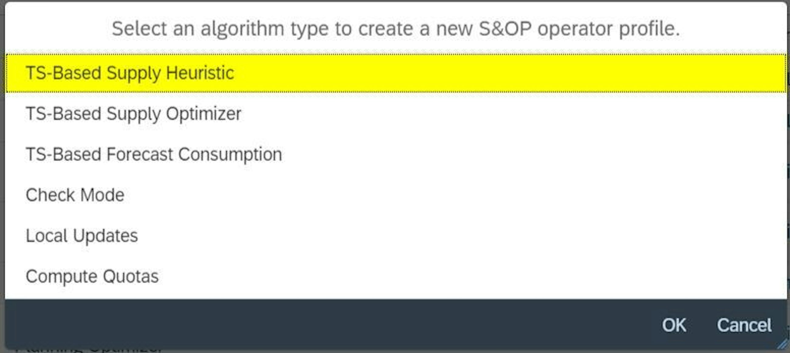
1. The finite heuristic: you can now create a constrained supply plan with this new heuristic type
Before 1911, the optimiser was the only standard way to automatically create a constrained supply plan in IBP (only available with the IBP Response and Supply license). This is no longer the case. With the 1911 upgrade, SAP has introduced a new heuristic type with which you are able to create a supply plan, taking certain supply and resource constraints into account.
The new finite heuristic
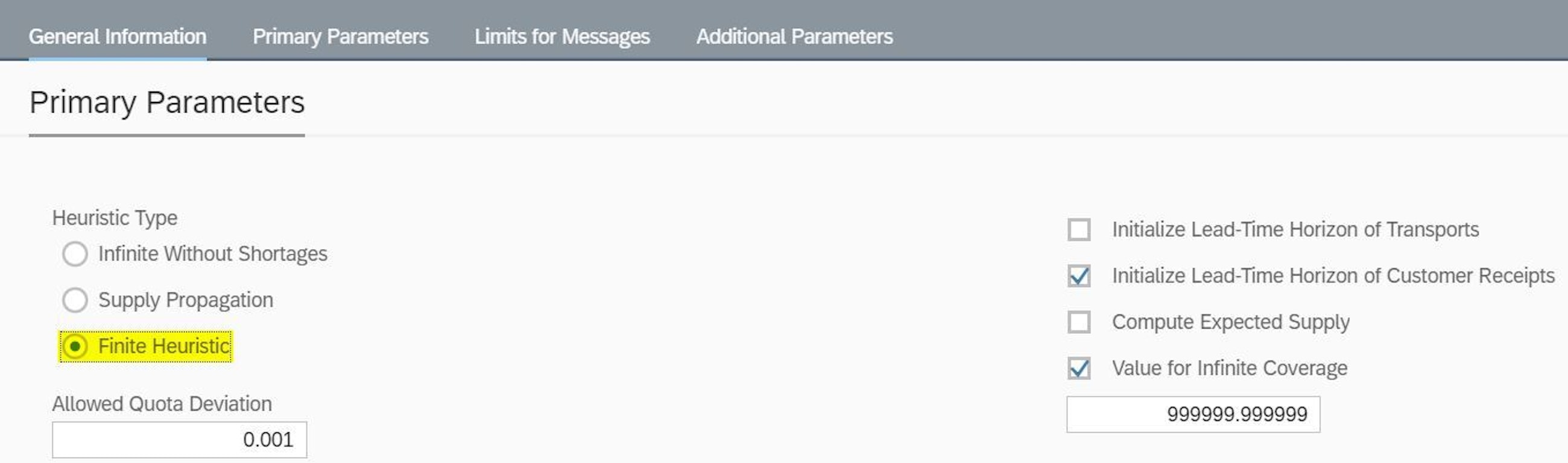
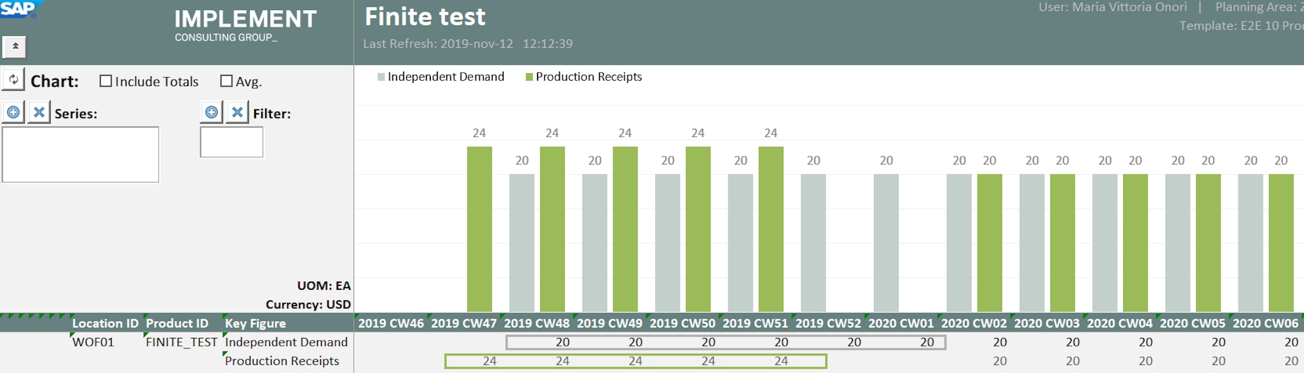
With this new so-called finite heuristic, you can create a supply plan based on priorities, and ‒ unlike the optimiser ‒ it prioritises demand over costs. So, how does it work? Basically, the finite heuristic uses different costs (e.g. non-delivery, late delivery, production etc.) that are traditionally used by the optimiser to determine priorities for demands to be satisfied and for sources of supply (e.g. production and transport) to be utilised.
For demands, the higher the cost of non-delivery, the higher the priority to satisfy the customer demand. On the supply side, the cost throughout the entire network is considered as costs are summed up along the supply chain to identify the least expensive path. Therefore, the higher the total costs (e.g. production, transport etc.), the lower the priority to use a certain path.
As of 1911, the finite heuristic has some limitations among which we find it worth mentioning that it does not consider time-dependent features such as costs, component coefficients, production outputs etc. Therefore, the heuristic uses the values of the current period and assumes that they are constant over the entire planning horizon. We expect to see this as well as other not yet supported features (e.g. lot sizing policies, resource capacity expansion, maximum and minimum receipts etc.) implemented in the coming releases – so stay tuned and be prepared to gain all the benefits of this new time series-based heuristic soon.
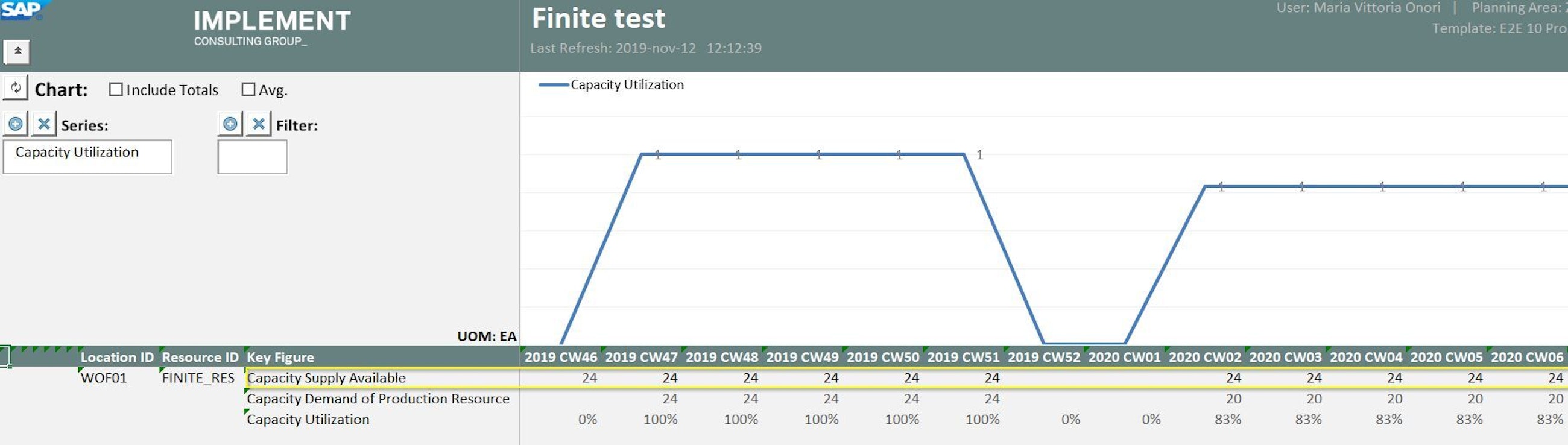
In this example, the finite heuristic respects the capacity constraint in weeks 52 and 1: quantities are produced in advance when there is available capacity.
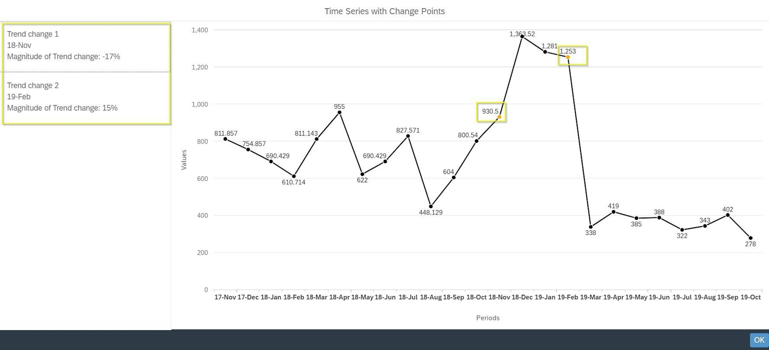
2. Change point detection: you can now automatically detect step changes and trend changes in your demand
Within demand planning, SAP has introduced a new functionality in the area of forecast automation: change point detection. With this functionality, you can identify significant changes with long-term effects in the time series.
You can detect both step changes (when the mean of the time series changes significantly) and trend changes (when direction or slope of a trend changes drastically).
For example, a step change may happen when a product is introduced to a new market, a competitor enters the market, or there is a change in the legal environment situation (e.g. a government stops subsidising a certain drug). Such changes often result in a higher (or lower) mean of time series values, which will be recorded by the system.
A trend change is identified when the change between two adjacent sections of the trend slope is either more than the minimum percentage defined or not large enough to meet the minimum requirement but when a significant step change can be detected between the sections.
For example, if there were a positive trend in the sales of Christmas decorations in November, and the trend continued with a much steeper slope in December when Christmas was much closer, the algorithm would identify a trend change in the time series. Or if the trend would continue with the same slope, but much higher values were registered in December, the algorithm would identify a trend change even though the slope did not change.
So, how can you work with change point detection? It basically requires two main steps:
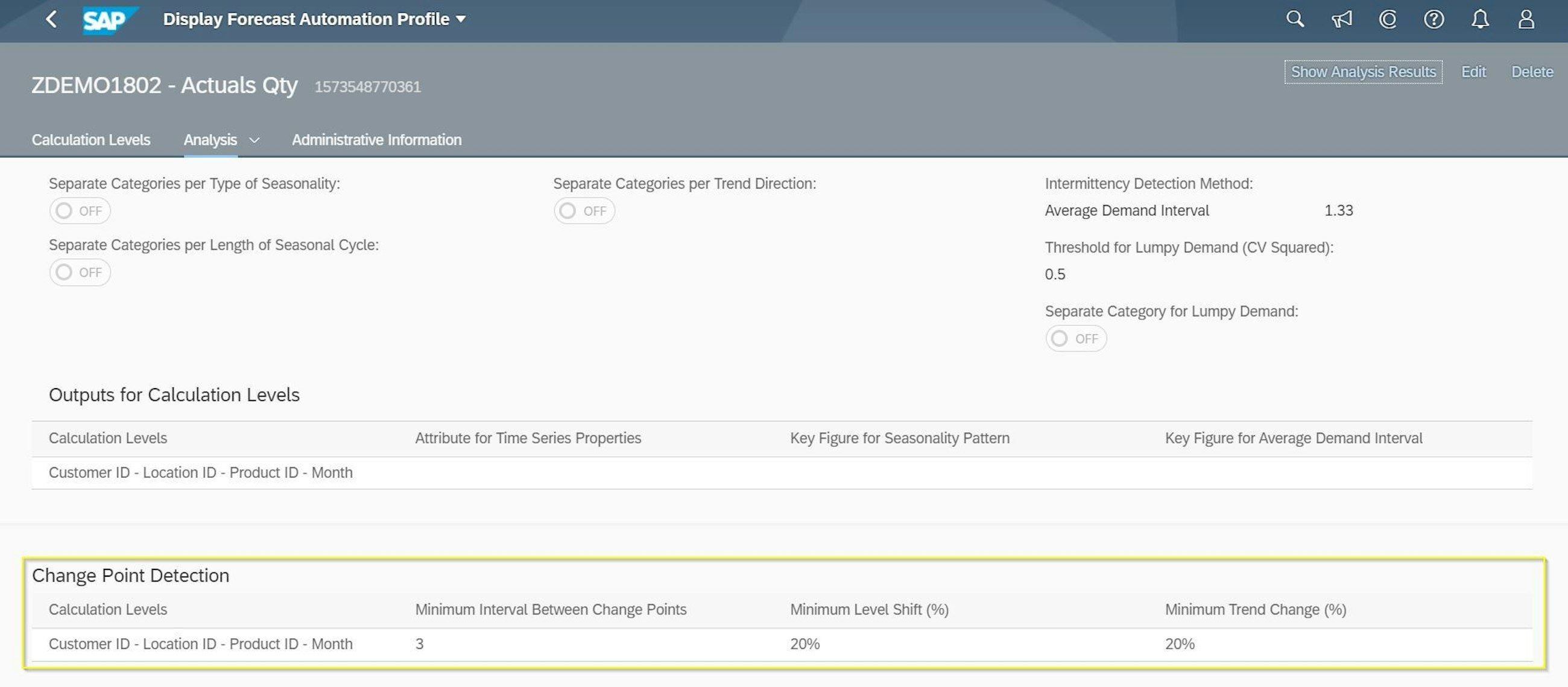
- You set up the rules for change point detection in the Manage Forecast Automation Profiles app. Here, you can specify thresholds to limit the number of change points that are identified.
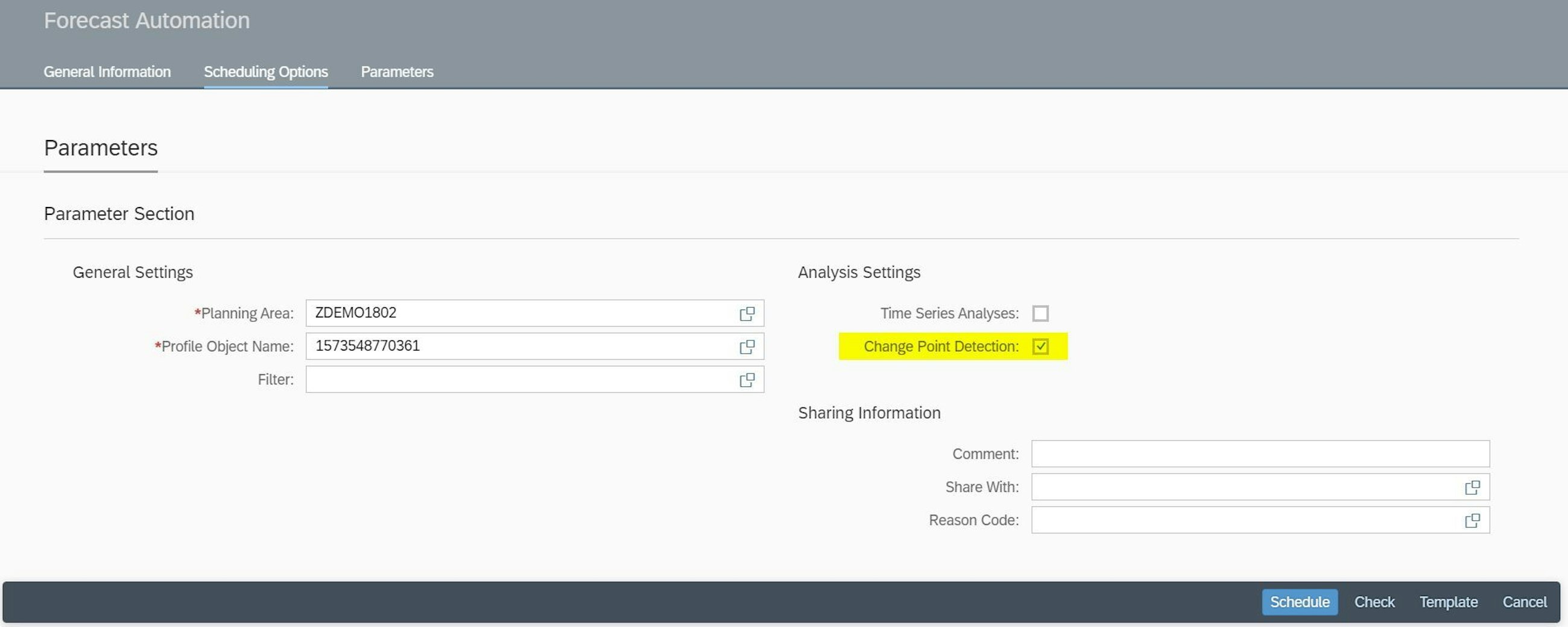
- You run a forecast automation job for which you select the Change Point Detection option.
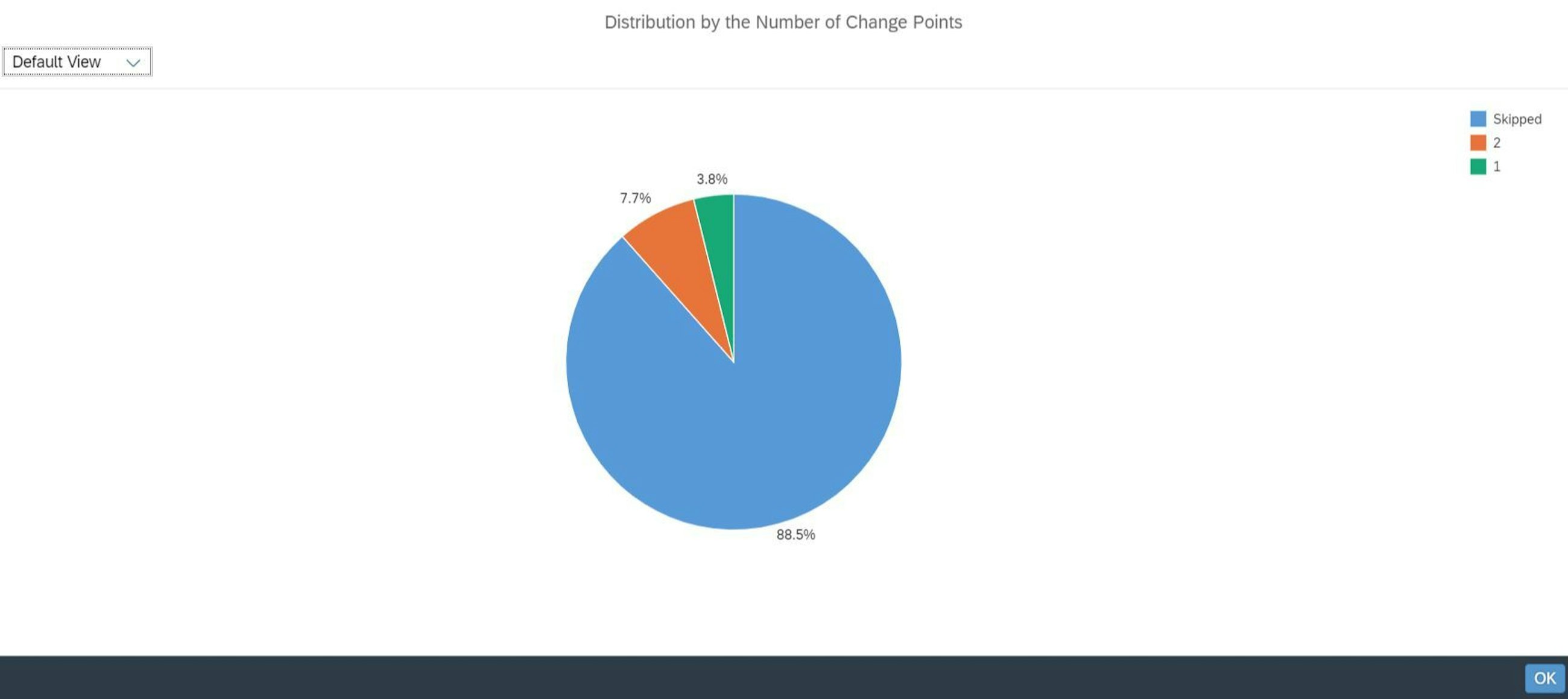
When you want to check the results of the forecast automation job, you can choose Show Analysis Results and then Change Points in the Manage Forecast Automation Profiles app. As a result, you will get a table that shows all planning objects that were analysed on the selected calculation level, the number of change points and the time series properties identified for each planning object.
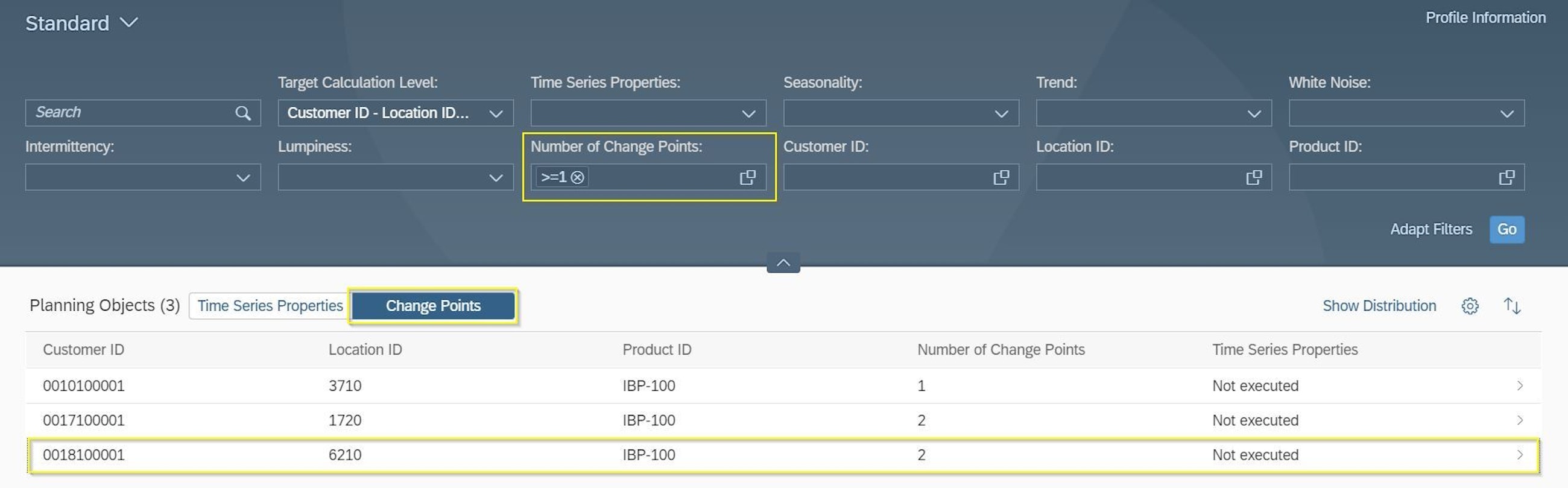
If you want to test this functionality, we recommend that you use the Show Distribution option, which shows how change points are distributed among the planning objects. Too many items with a high number of change points could mean that the configured thresholds may require some adjustment.
One thing you must remember is that if a step change and a trend change are both identified in a time series, the analysis will only register the trend change. Also, change points can currently only be used as information. Demand planners need to use this kind of information to understand why certain forecast models can predict the future less accurately and, most importantly, to actively adjust the forecast so that it considers the expected demand changes.
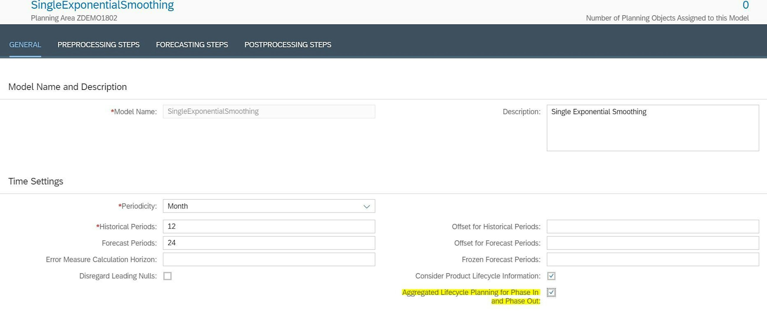
3. Aggregated lifecycle planning: you can now plan product phase-in and phase-out on an aggregated level
Up to this release, you could only use lifecycle capabilities if the forecast was being executed on a detailed level (SKU level) as launch and phase-out dates are maintained on individual products. Now, you can work with lifecycle planning for phase-in and phase-out on an aggregated level. So, if you run your forecast on e.g. product family level, or any other level that is more aggregated than SKU, the forecast will be adapted to account for the relevant phase-in and phase-out products belonging to that aggregated level.
For example, if you run the forecast on a product family and country level in your business, and you have a new product being introduced in March 2020 in a certain country within Product Family 1, the system will first execute the forecast on the defined aggregated level. It will then disaggregate the forecast between the new product and the existing products, and it will finally remove values in the months prior to March for the new product.
When you want to use this functionality, you just need to switch on the “Aggregated Lifecycle Planning for Phase-in and Phase-out” in your forecast model as it will be switched off by default due to performance reasons.
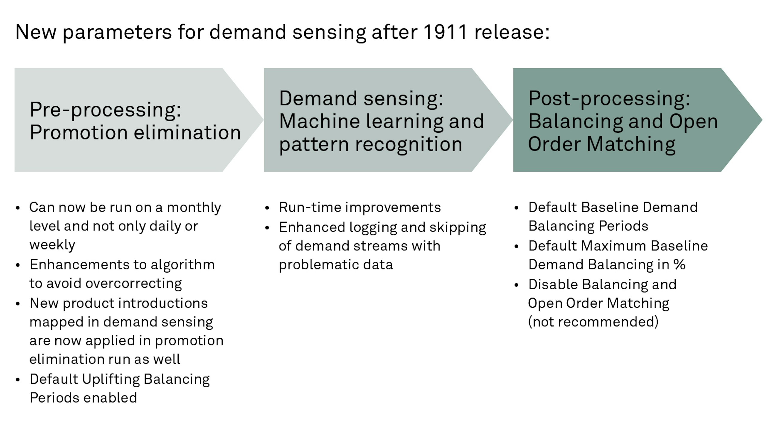
4. Demand sensing: you can now increase your daily forecast accuracy with new parameters to fine-tune the demand sensing algorithm
The demand sensing algorithm has been improved continuously since we implemented it for the first time for a client back in 2016. In the 1911 release, SAP has introduced some new default parameters as well as made it possible to run the promotion elimination on a monthly level.
One of our clients who currently uses IBP demand sensing has the following comments regarding the improvements from the 1911 release:
“Before the 1911 release, it was necessary to maintain balancing periods on a detailed level. This is doable if you have few planning combinations. But for some of our products we sell out of more than 50 locations, it will require a lot of maintenance. With Default Uplifting Balancing Periods and Default Baseline Demand Balancing Periods enabled, it is much more efficient to create a default balancing period which is relevant for the majority of the planning combinations and then maintain the exceptions on a detailed level for those combinations that require other periods. This offers a great flexibility and at the same time it is easier to fine-tune the algorithm. We expect this to improve our daily forecast accuracy further when using both Default Base Balancing and Default Uplift Balancing.”
We agree with the client and would like to go a bit more into detail with the new parameters in the following sections.
The pre-processing step, promotion elimination, is important to estimate the baseline sale. The baseline sale without promotion is the input for the demand sensing algorithm. Therefore, the better the input is, the more accurate the demand sensing result will be.
If promotions are on a daily level, they will be aggregated to a weekly level during the run, and weekly sales are cleansed from promotional impact. Now you can specify for how many weeks backwards and forwards this aggregation should take place with the new parameter “Default Uplifting Balancing Periods”. This is an important setting for companies in which a planned promotion can affect the sales both the week before the promotion and the week after the promotion.
From this release, you can also run promotion elimination on a monthly level. If this is the case, the Uplifting Balancing Periods are not taken into account as the promotions are then aggregated within the same month, and sales are then cleansed from promotional impact.
SAP has also made significant improvements to the post-processing step with the balancing and matching of open orders. Here, you can specify how many weeks backwards and forwards you should take forecast consumption into account when balancing baseline demand. This is done by analysing patterns of oversell/undersell situations.
The use case for this could be that you have a big planned promotion in week 3 and unusually high open orders in week 4. If the Default Baseline Demand Balancing Period is 1 or higher, the unusually high open orders will consume the planned promotion in week 3. Furthermore, you now have the possibility to set a percentage of how much the baseline balancing logic is allowed to consume of the first and last week within the balancing periods to avoid periods with zero sensed demand even though open sales orders have consumed the full forecast.
Also, you can now completely disable this balancing and matching of open orders. However, we would not recommend this unless you are already using a sophisticated forecast consumption logic built into your supply planning process that uses sensed demand as input.
5. Global inventory optimisation: you can now improve your inventory plan with a better phase-out plan during demand ramp-down and phase-out of products
When you run the global inventory optimisation, the algorithm has been improved with automatic detection of periods where demand ramp-down is taking place. A new key figure indicates when a period is detected when the demand falls below a defined threshold compared to the demand moving average. It is not considered a demand ramp-down until the period exceeds the exposure periods, lead time plus review period.
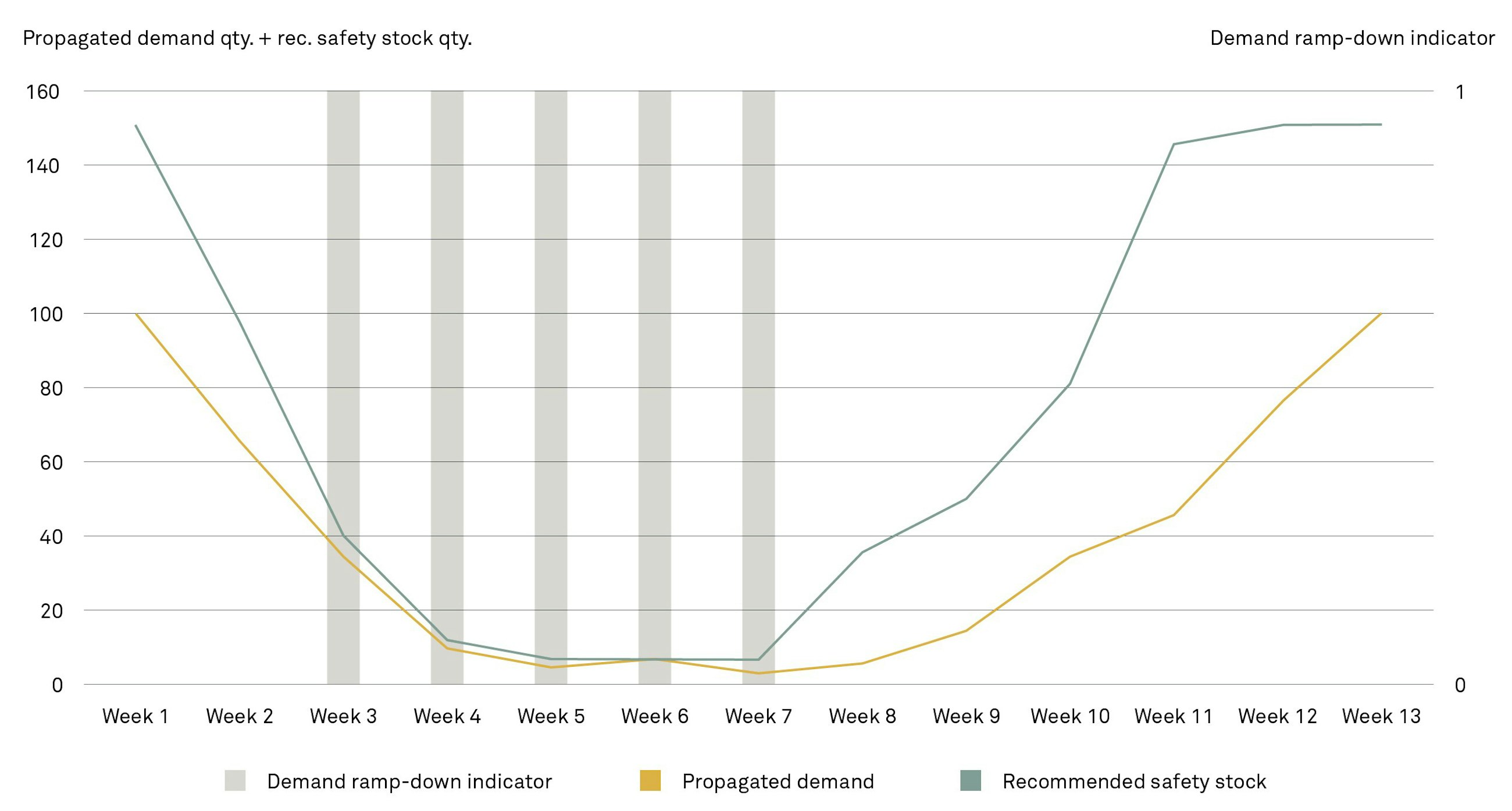
Besides indicating where a demand ramp-down is taking place, the algorithm detects when all consecutive periods have zero demand and adjusts the inventory target accordingly. You can use both features to help reduce the net working capital and avoid potential scrap when a product is being phased out.
For companies using inventory planning in SAP IBP, a new welcoming feature is also introduced. You can now use the attribute filter in the planning view in Excel for the inventory optimisation when doing simulations and scenarios. This will significantly reduce the run time and memory usage and improve the usability of doing scenarios and simulations with the global inventory optimisation algorithm.