Article
Five selected features of the 2111 upgrade of SAP IBP

Published
21 November 2021
In November 2021, SAP released the 2111 upgrade of SAP Integrated Business Planning (IBP). Just as the previous releases, we have compiled a staff-picked list of five features of the IBP 2111 upgrade that we think your company can benefit from and that can leverage your supply chain planning to the next level.
Five selected features of the 2111 upgrade of SAP IBP
1. Let the machine learning algorithm consider holidays and special events
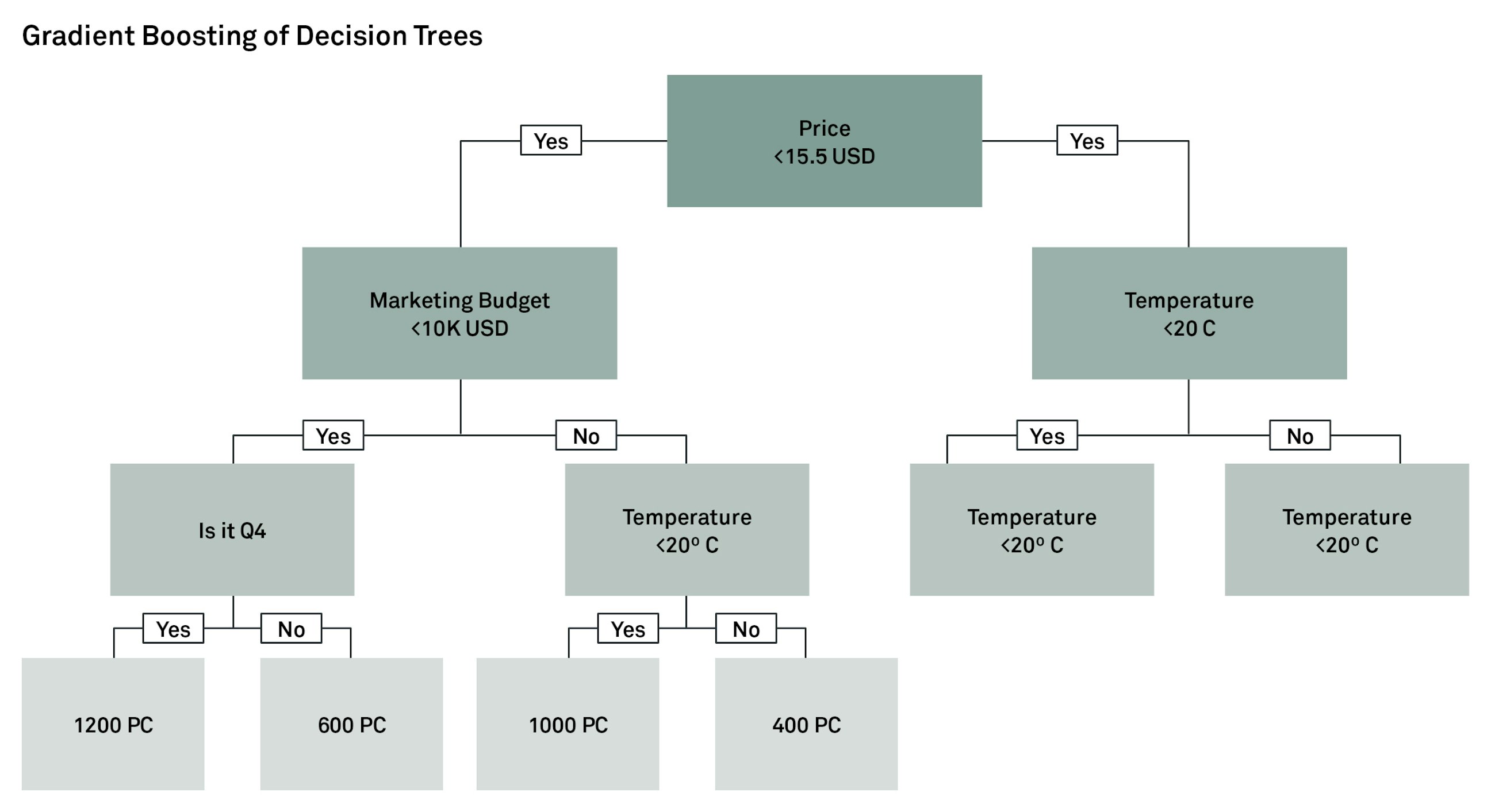
New and additional functionalities are continuously added to the machine learning capabilities in SAP IBP with the newest in line being the option of setting the gradient boosting of decision trees algorithm to calculate the impact of independent variables on the forecast and the ex-post forecast. Gradient boosting can be useful in demand planning when several external conditions need considering during the forecast calculation. With the new added functionality, a demand planner can run the analysis both on categorical and non-categorical variables.
The categorical variables allow the algorithm to learn from past events, e.g. if the sales pattern for a given product is connected to events in the past, e.g. extraordinary sales for religious holidays like Easter or Ramadan etc. or sport events which do not happen at the same date every year. These periods can then be marked with a categorical variable and the Gradient Boosting algorithm will then learn itself to move the extraordinary event to next time the categorical variables will happen.
If you define a categorical variable for the holidays, you can choose to save a number such as 100 in it for Easter and 200 for Ramadan, and the algorithm will interpret that number as a code, not as a value. It will learn that the event with the code 100 increased the sales values by 20%, and for event code 200 increased sales by 25% in the period when it occurred, and it will forecast correspondingly higher sales values for future periods with the same code. Keep in mind that you need to use the same event codes for e.g. Easter every year.
We do not recommend using the Gradient Boosting forecast model for products with high variation in demand, because it easily overfits the training data, meaning that the forecast may correspond too closely or exactly to the sales history and may therefore be less reliable. And the model cannot make good predictions for cases where the future values of independent variables largely differ from the corresponding past values.
2. New machine learning algorithm: Demand sensing with gradient boosting (FULL)
The newest IBP release from SAP includes a new forecasting algorithm: Demand sensing with gradient boosting (full). This new algorithm is like the gradient boosting of decision trees algorithm and is a machine learning algorithm that can consider all the information gained from each independent variable when it is calculating the sensed demand. This new algorithm is only available for full rounds of demand sensing and not for updates.
The algorithm performs repeated optimisation on several decision trees in a tree-like model of decisions and possible consequences and these together are combined into an ensemble model determining which extra signals that should be considered at which level of the tree structure during the final calculation of the sensed demand. Thus, the new model takes the best of the elements from the Gradient Boosting of Decision Trees model and combines this together with demand sensing.
With this new algorithm, there some clear advantages and considerations that must be taken into account before including demand sensing into the forecast model used in your supply chain.
Advantages:
- The calculation and result of the Demand Sensing with Gradient Boosting is more accurate than a regular demand sensing run, which consider the extra signals in the order that they have been added to the forecast model.
- The Demand Sensing with Gradient Boosting does not require open orders as input to the algorithm run and thus more flexibility is added.
- With Demand Sensing with Gradient Boosting you can decide if you want to use historical or both historical and future extra signals when running the forecast algorithm.
Considerations:
- The tree structure is difficult to perfect and depends on a lot of training data to make the algorithm make good predictions for cases where the future values of independent variables significantly differ from any corresponding past value.
- The Demand Sensing with Gradient Boosting algorithm does require a lot of computing, which in turn can increase the execution time of the planning run.
- To make the algorithm work properly it requires weekly optimised sensed demand as input to the planning run. Furthermore, there is currently no change point detection or trend shifts included in the current algorithm.
The new thing added to the demand sensing algorithm is the Gradient Boosting of Decision Trees, which is a method to calculate the impact of independent variables on the forecast. Based on five different proofs of concept generated by SAP, it is identified that the forecast accuracy is improved by up to 35% compared to using the normal demand sensing. Thus, this can be a case to look into if you are already using the demand sensing algorithm in your current planning run.
An example of how gradient boosting is affecting the decision of the demand based on temperature and marketing budget.
3. Location product substitution now works with finite heuristic enabling even better satisfaction of customer demands
The new upgrade for SAP IBP 2111 offers an enhancement to the location product substitution functionality. The feature is now also relevant for the finite heuristic ensuring that the customers are satisfied with an alternative product when aiming for creating a feasible and constrained supply plan.
Location product substitution is not a new functionality as we wrote about this in our article “New Features of SAP IBP 2008” where we briefly presented the functionality and how it works. For the ones that did not read that article, we will in this section introduce both the location product substitution functionality and the finite heuristic. At the end, we will introduce the benefits of using this together with the finite heuristic and what you must do to get started with this.
The finite heuristic is a heuristic that can provide a finite demand and supply plan, which is based on a prioritisation of demand while still considering the supply and resource constraints that are maintained in the system. The prioritisation for the demand is performed by adding the costs to the demand where the higher cost of non-delivery/late delivery results in a higher priority for the demand. Similarly, the costs added to the sources of supply works in the way that the finite heuristic will go for the lowest cost source of supply. Thus, it seeks to provide the cheapest option for producing/delivering the product. By doing this, you can as a planner create a supply plan based on priorities for demand and thus directing your available capacity towards the products that generate the highest revenue.
Now that we have knowledge of the finite heuristic, we can start digging into the location product substitution, which is a cool feature when demand for customers can be fulfilled by multiple products.
Location product substitution is a functionality that enables you as a company to substitute any leading product where a supply shortage is present with another substitution product. This could be relevant when promoting a product series or introducing or discontinuing a product. By using the functionality you can ensure a smooth discontinuation of an “old” product and introduction of the “new” product. This feature can both be used for customer demands and for dependent location demands. The location product substitution functionality is now available for all heuristics in the SAP IBP suite, but of course with different settings for the master data and key figures needed to be maintained.
Now that we both have the knowledge of the finite heuristic and the location product substitution, we can introduce the functionality and how this can help us in satisfying the demands of our customers in the future.
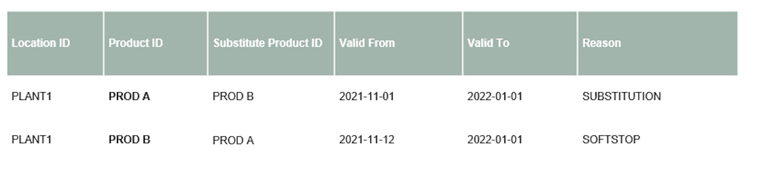
For the location product substitution to work we need to maintain some substitution master data, which is simple to maintain. One thing to bear in mind is the reason codes which are predefined from SAP and which have to be maintained for the substitution to work. Furthermore, it is important to maintain a “valid to date” if we do not use HARDSTOP as a reason code for the substitution.
Creating the location product substitution master data is easy to do. One thing to bear in mind is the reason codes that must be fulfilled.
Once this master data is maintained in the IBP system, you run your finite heuristic and it is now possible to see the result of substitution products through the substitution key figures for supply and receipts.
Once the master data is created, it is possible to see how the product substitution works with Prod B substituting the shortage of Prod A demand.
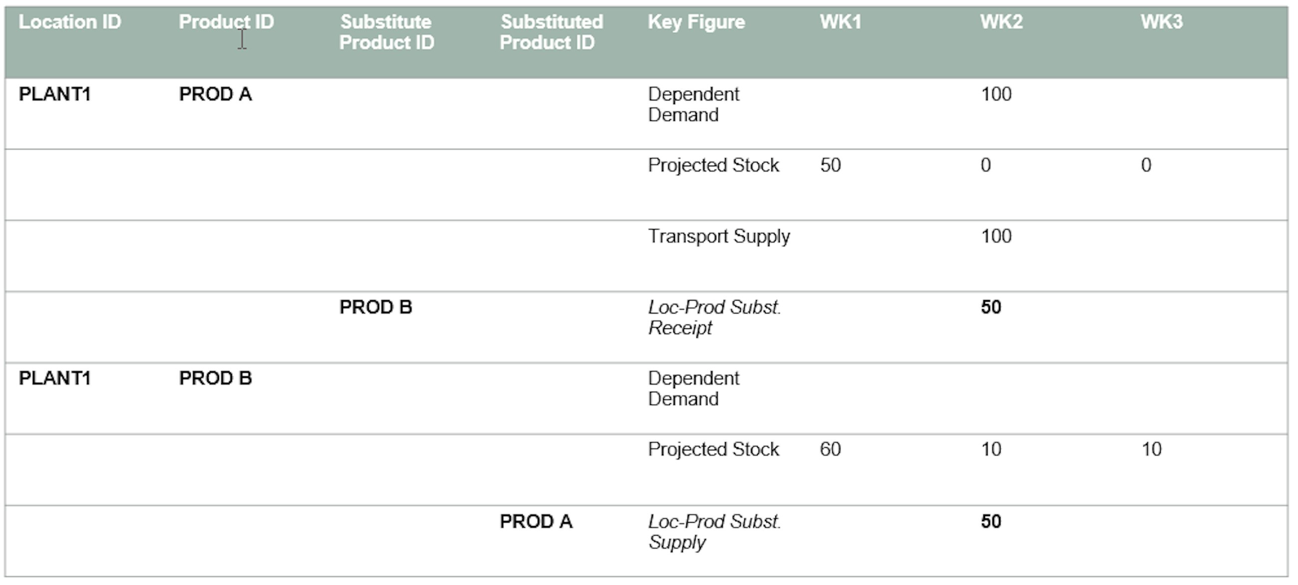
Looking at our example of location product substitution, it is possible to see that we have a location (Plant 1) which provides both Prod A and Prod B to a specific customer. As can be seen from the picture, the demand of 100 units is on Prod A and Plant 1 has 50 units in stock. However, as Prod B is a substitution product for Prod A, we can utilise the available stock of Prod B of 60 units for supplying the customer demand of Prod A. The quantity delivered of Prod B to the demand of Prod A is seen in the key figure Loc-Prod Subst. Receipt where we can see that the entire stock of Prod B is supplied to Prod A’s demand.
This new feature can be very useful for the planners when promoting products or introducing new products to the market. It is simple to set up in the IBP system in terms of master data and requires minimal configuration changes to both new master data types, attributes and planning levels. The only thing to remember with this functionality is still that this only works for 1:1 substitution and if you want to use multiple location product substitution this needs to be done through the Supply Planning Optimizer instead.
4. Enhancements in Planner Workspaces: The future web-based planning for SAP IBP
With the newest release of SAP IBP 2111, even more features have been added to the Planner Workspaces, highlighting even more that this is the future web-based planning module of SAP IBP. From the 2105 release, we received the Planner Workspace functionality in its basic form where it was possible to create a planning view that could easily be shared across departments and roles in the business. The functionality was basic with alerts being included, performing simulations and creating scenarios and scheduling jobs in the Planner Workspaces. With the new upgrade, SAP has added even more functionality to the Planner Workspaces making it more attractive for the simple planning tasks to be performed in the Fiori instead of performed through Excel.
The new features added to the Planner Workspaces include:
- Analytics charts: where the data can now be presented in a chart format.
- Simulations of changes to key figure values and sharing these with other planners.
- Creation of planning notes to capture information and share this with other planners.
- Attributes linked to an ID attribute can now be displayed in Planner Workspaces.
- Setting ad hoc parameters when scheduling application jobs based on templates.
The three primary features that have been added to make the Planner Workspace even more useable are the analytics chart, the application jobs creation within the app and the scenario functionality.
For the analytics chart functionality, it is quite like the functionality used when creating a dashboard. First, the analytics chart is created in the “Analytics Chart” app. Then it is added to the Planner Workspace planning view.
Assigning charts to Planner Workspace is similar to adding it in a dashboard.
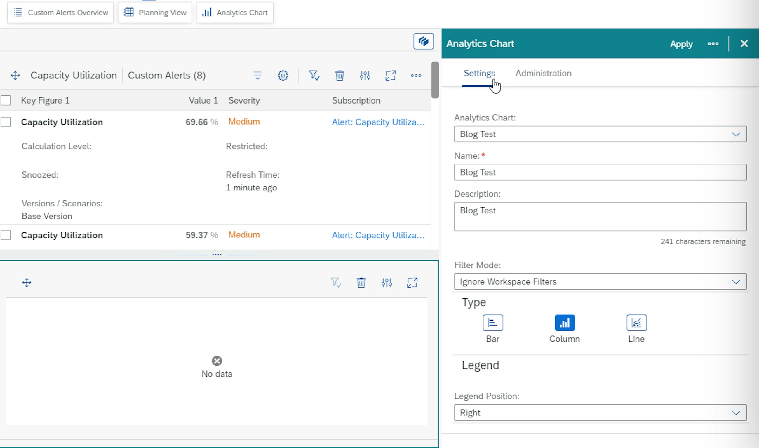
The only thing to bear in mind when adding the chart is whether to apply the filters of your Planner Workspace to the analytics chart.
The graphs that can be used are similar to the ones in Analytics Charts
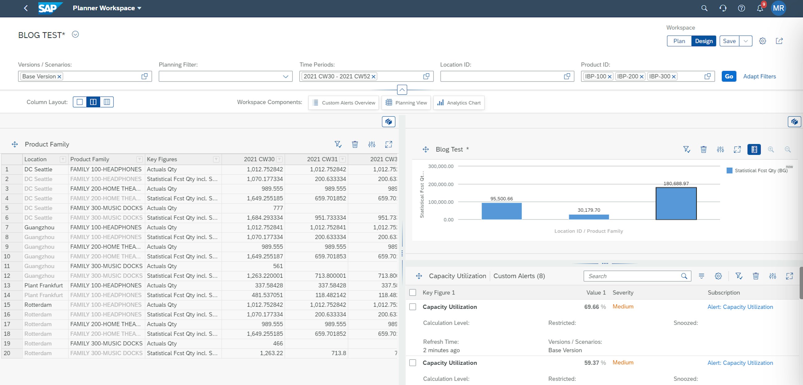
By adding these charts, it has become easier to generate an easy overview of the planning tasks at hand and extract the relevant planning information needed to make the right decisions – all this while having the planner as the driver of the planning tasks. This makes the Planner Workspace even more personalised and intuitive for the planners making the daily tasks.
Another added feature is the ability to schedule application jobs through Planner Workspaces. The new enhancement provides the ability to run the application job through an assigned Application Job Template.
In Planner Workspaces, you can now see the status or run the application job.
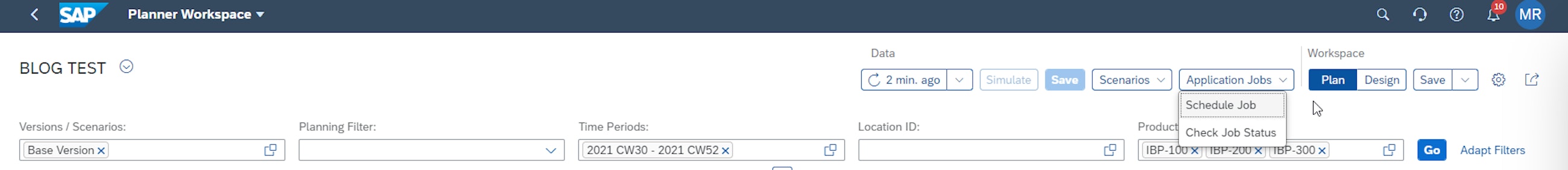
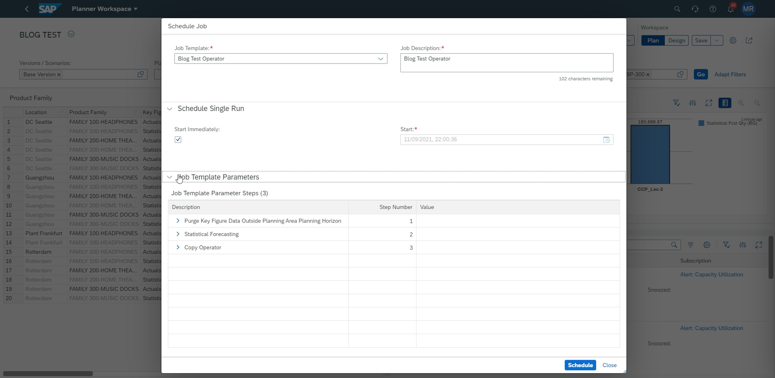
When an application job is run, this is chosen from the drop-down menu where all the available templates for the planning area are present. From this it can be decided if this is to be started right away or scheduled in the future. Furthermore, it is possible to see the steps in the template process.
The Application Job template and steps can be seen in the scheduling function.
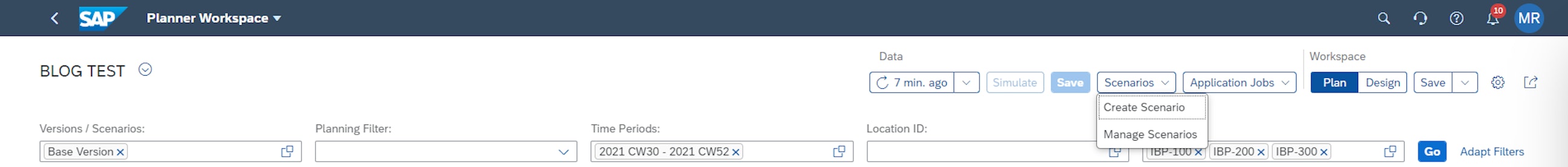
The last feature which has been added to the Planner Workspaces is the Scenario functionality. This is added to compare results and what-if analyses across different scenarios and identify the impact of supply chain changes, which in turn increases the transparency of the stakeholders taking the planning decisions. Creating and managing a scenario in Planner Workspaces is not the only feature added as you now also can delete and promote the scenarios as well, which will be seen instantly in the Excel Add-In of the IBP solution for other planners.
Creating a scenario is just a click away in Planner Workspaces.
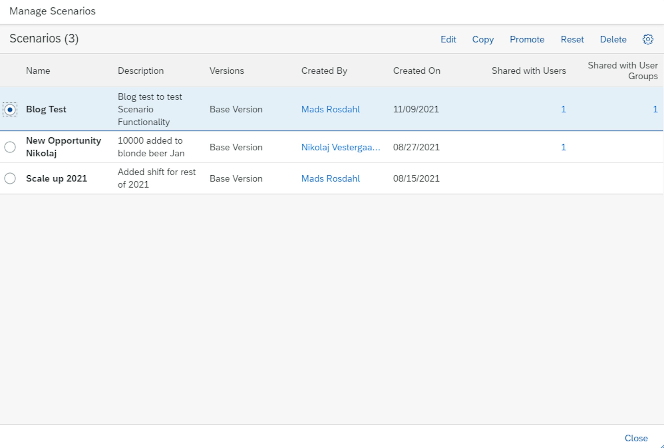
Once the scenario has been added, it is easy to compare the different numbers in Planner Workspaces and from there it is possible to either edit, copy, reset, delete or promote the scenario directly through the Planner Workspaces.
In Planner Workspaces, it is easy to manage your scenarios just as through the Excel Add-In.
With some of the new features of SAP IBP 2111, it has become even easier for IBP users who have no need to perform advanced analyses or planning in Excel to use the IBP tool. In the future, SAP is investing even more in improving the functionality of the Planner Workspaces and is adding the following features to Planner Workspaces:
- Q1 2022: Adding interactive planning to Planner Workspaces (ability to change orders directly in Planner Workspaces and identifying dependent changes to the current planning session).
- Q3 2022: Increased flexibility in application job triggering from Planner Workspaces.
- Q3 2022: Features to be added to Planner Workspaces that will allow for planning across SAP IBP and PP/DS (Synchronized Planning).
5. Use machine learning functionality to create your segmentation
In our 2105 blogpost, we wrote about the introduction of the K-means for segmenting products with similar characteristics, and this has now been further enhanced. The ABC/XYZ segmentation has for a while had the function of creating segments based on grouping, which for example can mean that the ABC analysis can happen for each market or country if the market or country is selected as the attribute for grouping. This means that a product in Market 1 can be a C product and in Market 2 an A product.
The K-means is a clustering approach that cluster products with similar demand patterns.
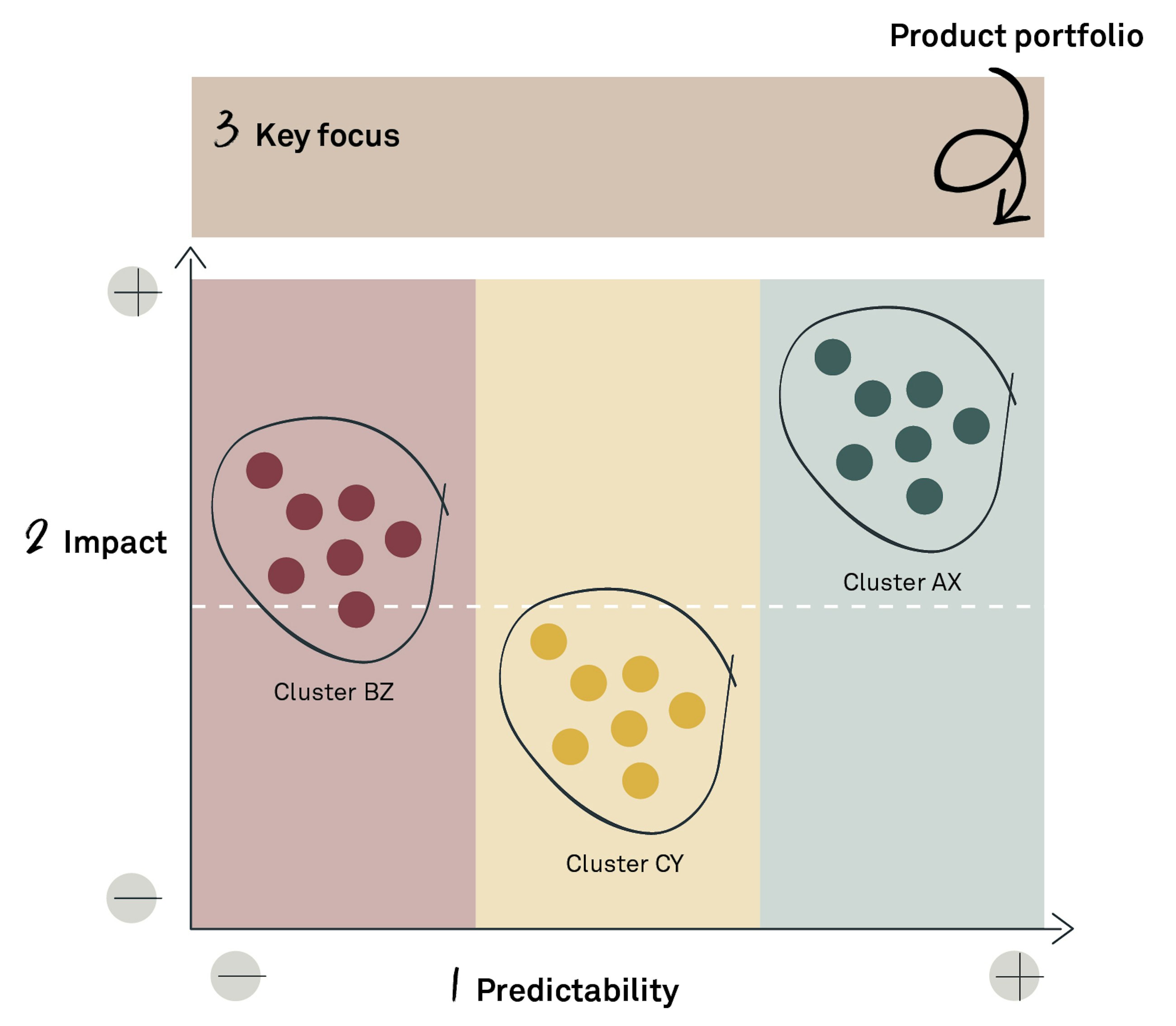
This functionality is now also enabled for segmentation with K-means. The K-means approach for clustering products is very helpful for grouping products with same sales patterns. However, we still find the Forecast Automation profiles and ABC/XYZ segmentation more useful when applying differentiated forecasting and planning approaches for them.
Read our previous blog posts 13


Article
Read more

New features of SAP IBP 2011
Five selected features of the 2011 upgrade of SAP IBP.Article
Read more

New features of SAP IBP 2008
Five selected features of the 2008 upgrade of SAP IBP.Article
Read more

New features of SAP IBP 2005
Five selected features of the 2005 upgrade of SAP IBP.Article
Read more

New features of SAP IBP 2002
Five selected features of the 2002 upgrade of SAP IBP.Article
Read more

New features of SAP IBP 1911
Five selected features of the 1911 upgrade of SAP IBP.Article
Read more