Article
Five selected features of the 2008 upgrade of SAP IBP


Article
Read more
1 September 2020
At the beginning of August 2020, SAP released the 2008 upgrade of SAP Integrated Business Planning (IBP). We have compiled a staff-picked list of five features of the IBP 2008 upgrade that we think your company can benefit from and that can leverage your supply chain planning to the next level.
What’s better than summer vacation? For demand planners, one answer could be the introduction of the new functionalities in the area of product lifecycle management. With these functionalities, you can now mass-upload reference material information from CSV files or enter it directly into the product lifecycle management application in Fiori.
This becomes handy when you introduce a new product range to the market, and you expect these products to have similar demand patterns as an existing range.
For phase-in products, planners often have difficulties making the forecast due to no sales history to be considered by the statistical forecast model, causing planners to often spend too much time on manual forecasting. By assigning weights to the historical sales from one or more products to a phase-in product, you can now in a much simpler way include multiple phase-in products in the statistical forecast calculations.
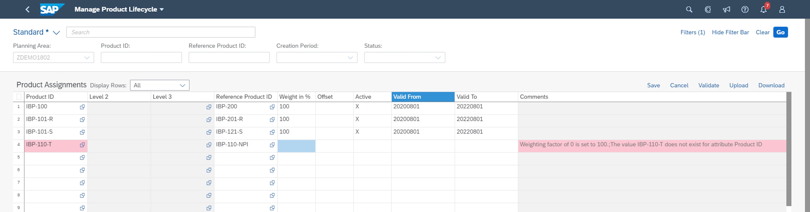
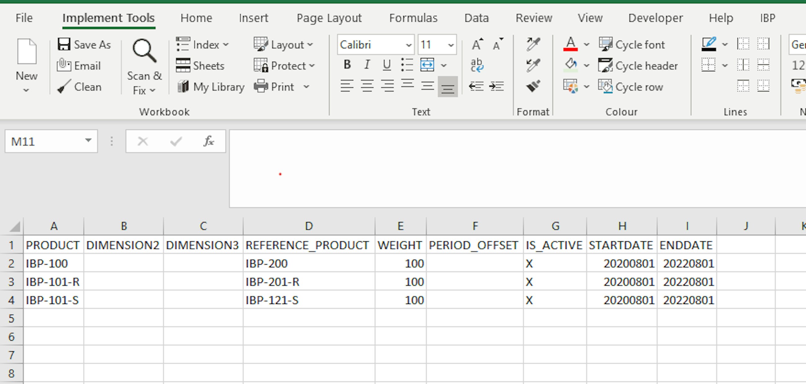
Before the 2008 upgrade, each product and their reference products had to be handled manually, however; with the introduction of the multiple product assignment, you can now handle this easier. It is now possible to create a CSV file outside IBP and upload the file to the system or fill out the product reference table in a much faster way than before.
So, how can you work with the new product lifecycle management enhancements? It basically requires three main steps:
Another added functionality to the multiple product assignment is the error detection, which shows if a reference product is nonexistent. Thus, the system will show an error message with the wrong reference material number.
In addition to the enhancements in the application, the 2008 upgrade also includes product lifecycle management for demand sensing. You are now able to use the product lifecycle references in the demand sensing forecast algorithms and through that include the phase-in and phase-out products in the short-term forecast.
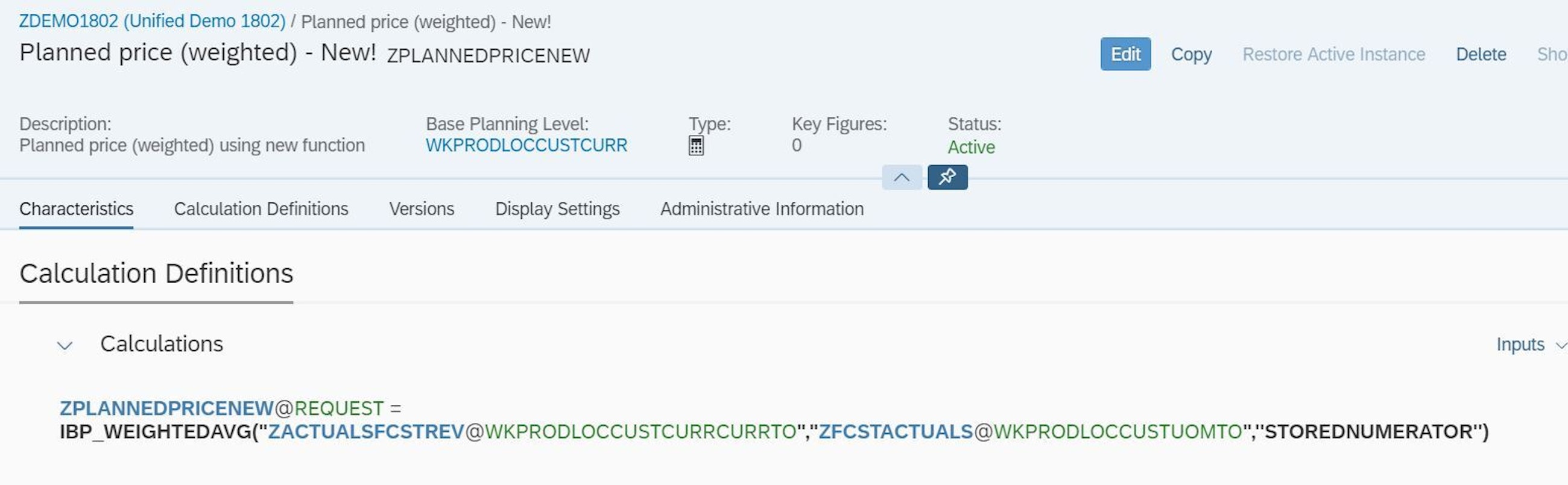
Much has been done in the area of model configuration over the last quarters, where many of the key functionalities delivered have aimed to improve key figure calculations. In the wake of the last releases, the 2008 upgrade does not disappoint and provides two new functions that simplify key figure calculations.
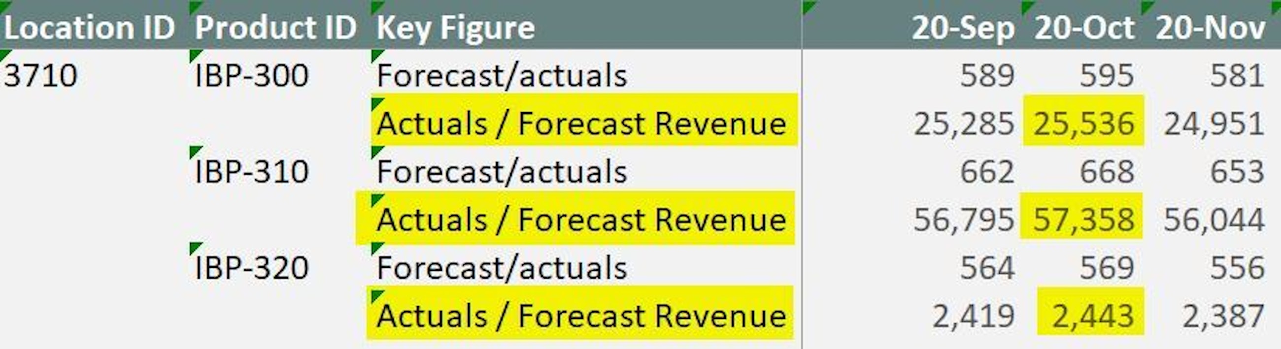
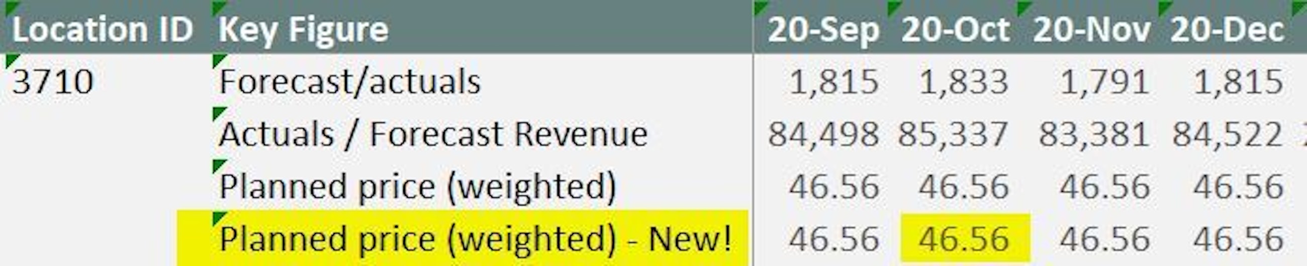
Before this release, creating a “weighted average” key figure required different intermediate calculations – now you can use the weighted average function to calculate the weighted average for a key figure in one single step – finally!
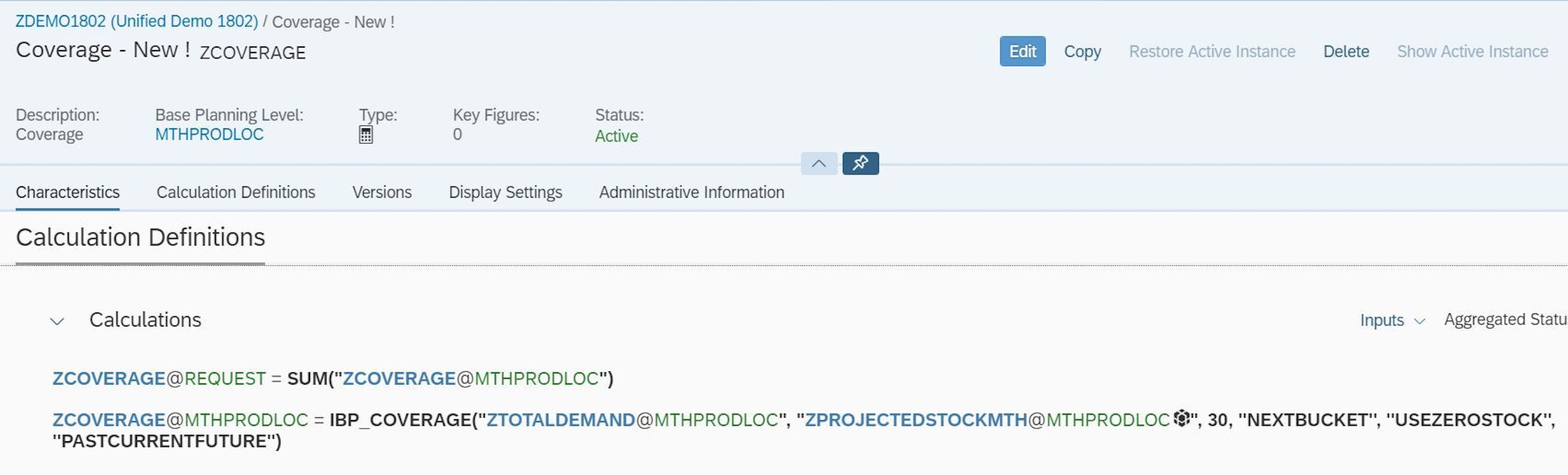
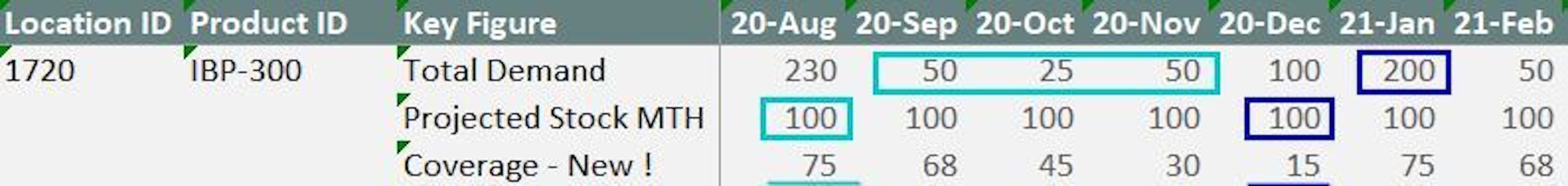
Up until this August, there was no standard functionality in IBP to calculate the days of inventory, i.e. how long the stock will last based on the current demand plan. With the new coverage function now available, you can easily calculate this KPI in a key figure, providing a simple way of determining how many days of planned demand can be covered by the projected stock.
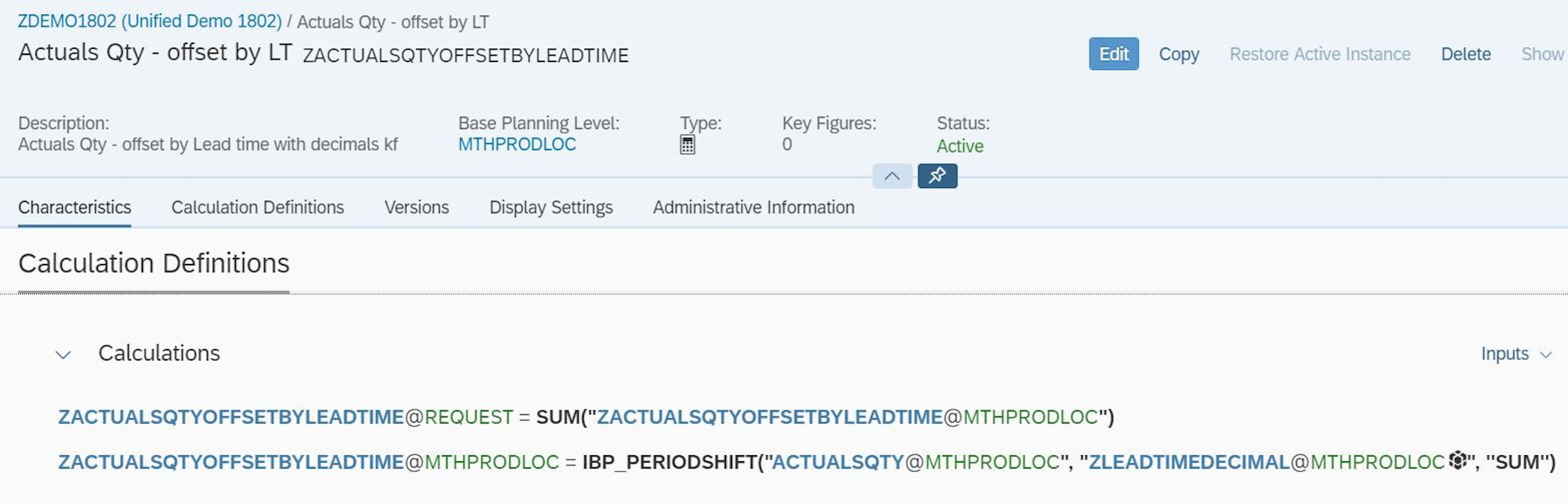
In addition to these two new features, the existing period shift function (IBP_PERIODSHIFT), which was introduced in the 2002 release, has been enhanced with a third parameter: the aggregation type. You should use this new optional parameter when you use a key figure to define the number of periods by which you want to shift the input key figure. In these cases, where you might end up with multiple values in a time bucket, you can now define how the key figure value should be calculated – possible values are SUM, MIN, MAX and AVG.
In case you are looking into how easily you can analyse and review your data, and you are already using the IBP dashboards, here are some great news.
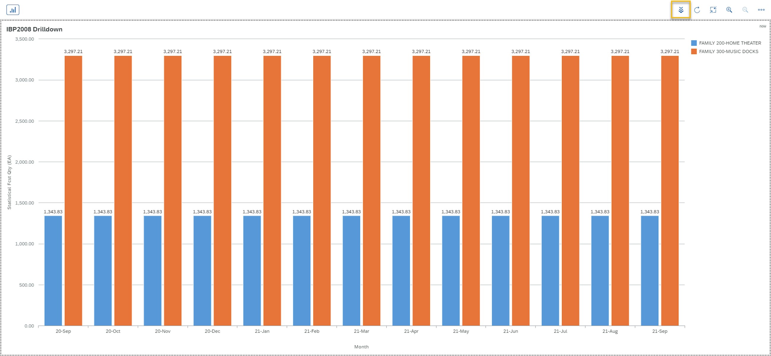
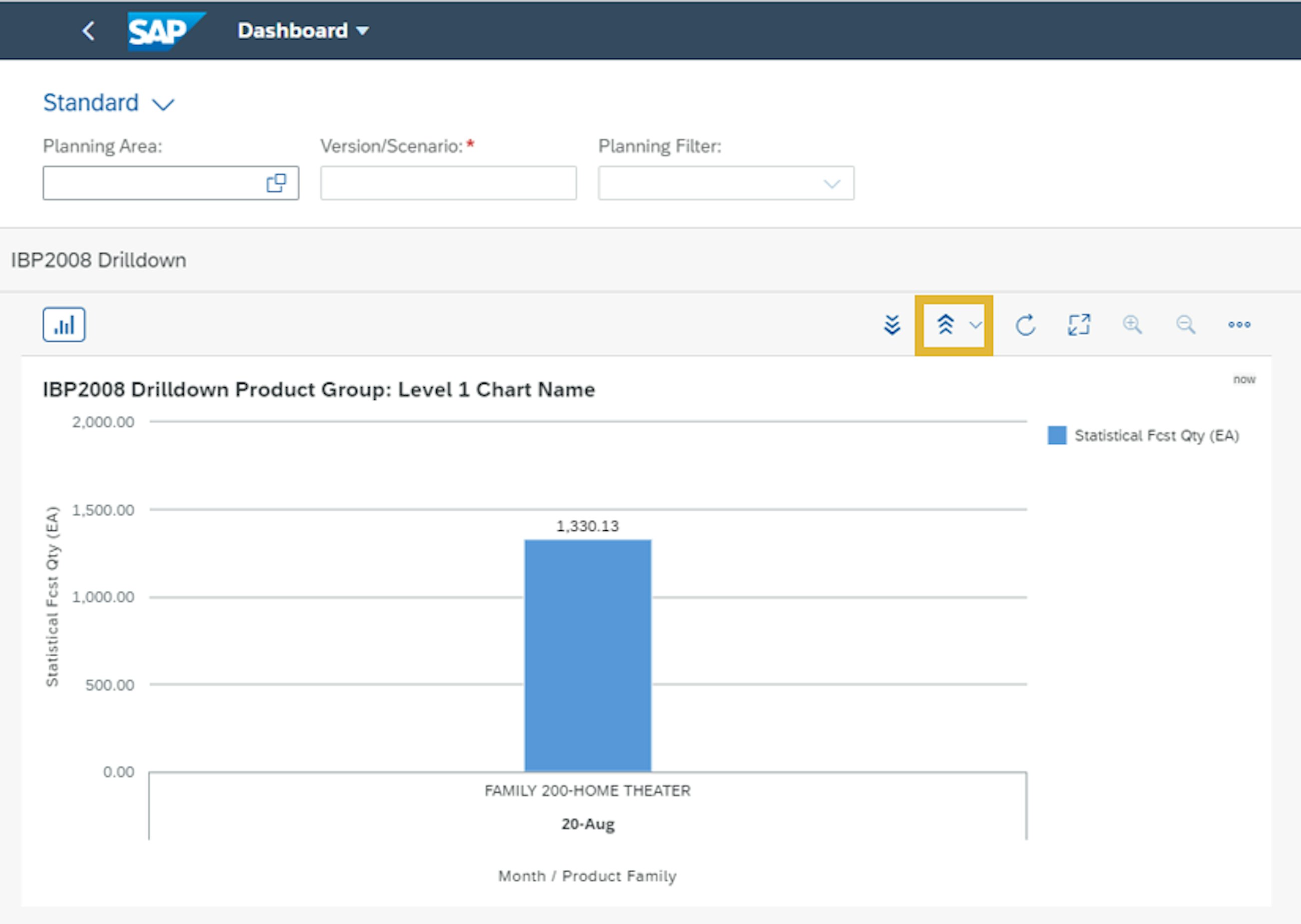
The dashboard functionality has been improved continuously since its introduction, and with the 2008 release, SAP has introduced improved drilldown functionalities and cascading filters in the dashboard application in Fiori. Before this release, you had to go to the analytics application to make a drilldown on your data, however; with the added functionalities, you can now drill down directly in the dashboard app.
You simply just select some data points on the charts and click on the drilldown icon. To enable this, you need to have created the drilldown path in the analytics app. If you have defined multiple paths to your drilldown in the chart, you can select which path you will follow directly in the dashboard.
Another added functionality which you can now use directly in the dashboard application is that you can now cascade ad hoc filters and planning filters to the next level while you drill down in the charts. SAP has included an option to decide if you want to cascade ad hoc filter and planning filter values to the next levels when creating the drilldown path. One example is that you can use the planning filters you have defined in Excel or in the planning filters app and use them to analyse your data in the chart where you did the drilldown.
SAP has also introduced the option to transport the dashboards and analytics via the transport model entities app.
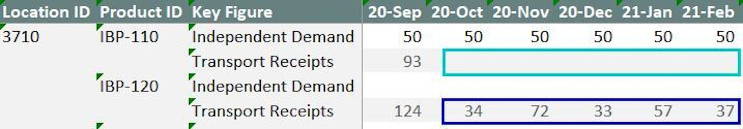
If product substitution sounds familiar to you in the IBP context, it is because there is an existing functionality for modelling substitute products: you can substitute a particular product or components by one or more identical products which have different product IDs (e.g. because of the plant at which they are produced).
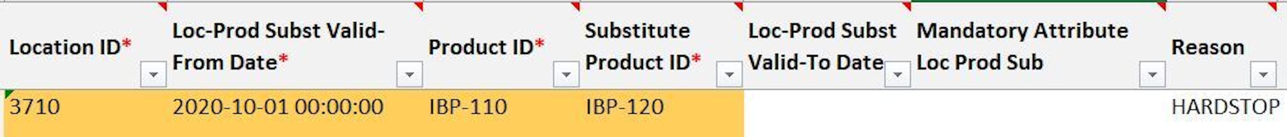
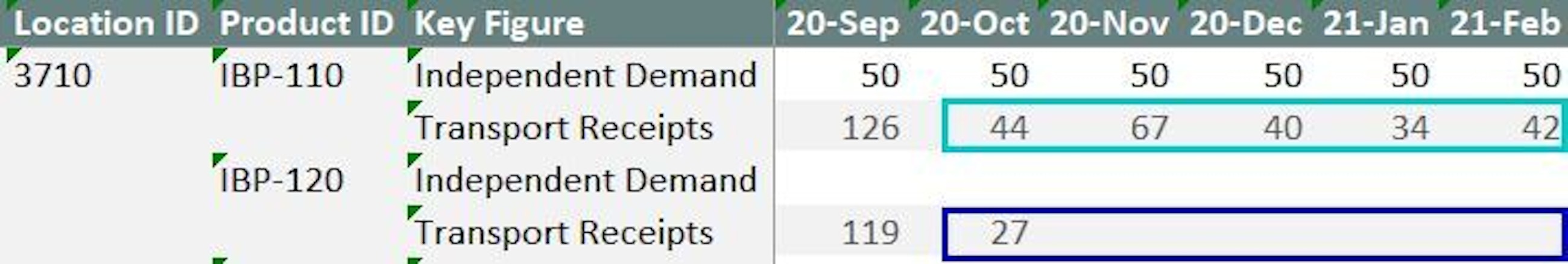
As you might have already guessed, the novelty of the recent location product substitution functionality is due to bringing the locations into the picture. With this new feature, the demand for a leading location product can be satisfied by supplying another (substitute) location product and vice versa. This new feature can be particularly useful when you plan for product discontinuation and product promotion.
When a product is being discontinued, e.g. because a newer model is being introduced in its place, you might want to stop supplying the “old” product even though you still have inventory. In other cases, you might opt for having a “use-up” phase, during which you want to keep selling the “old” product from the remaining stock to avoid waste.
Another scenario in which you might use this functionality is when you want to run a promotion campaign to boost the sales of a product. In this case, you might want to sell an alternative product instead of the leading one for a limited period of time. During this promotion phase, you might even want the demand for the original location product to not be satisfied.
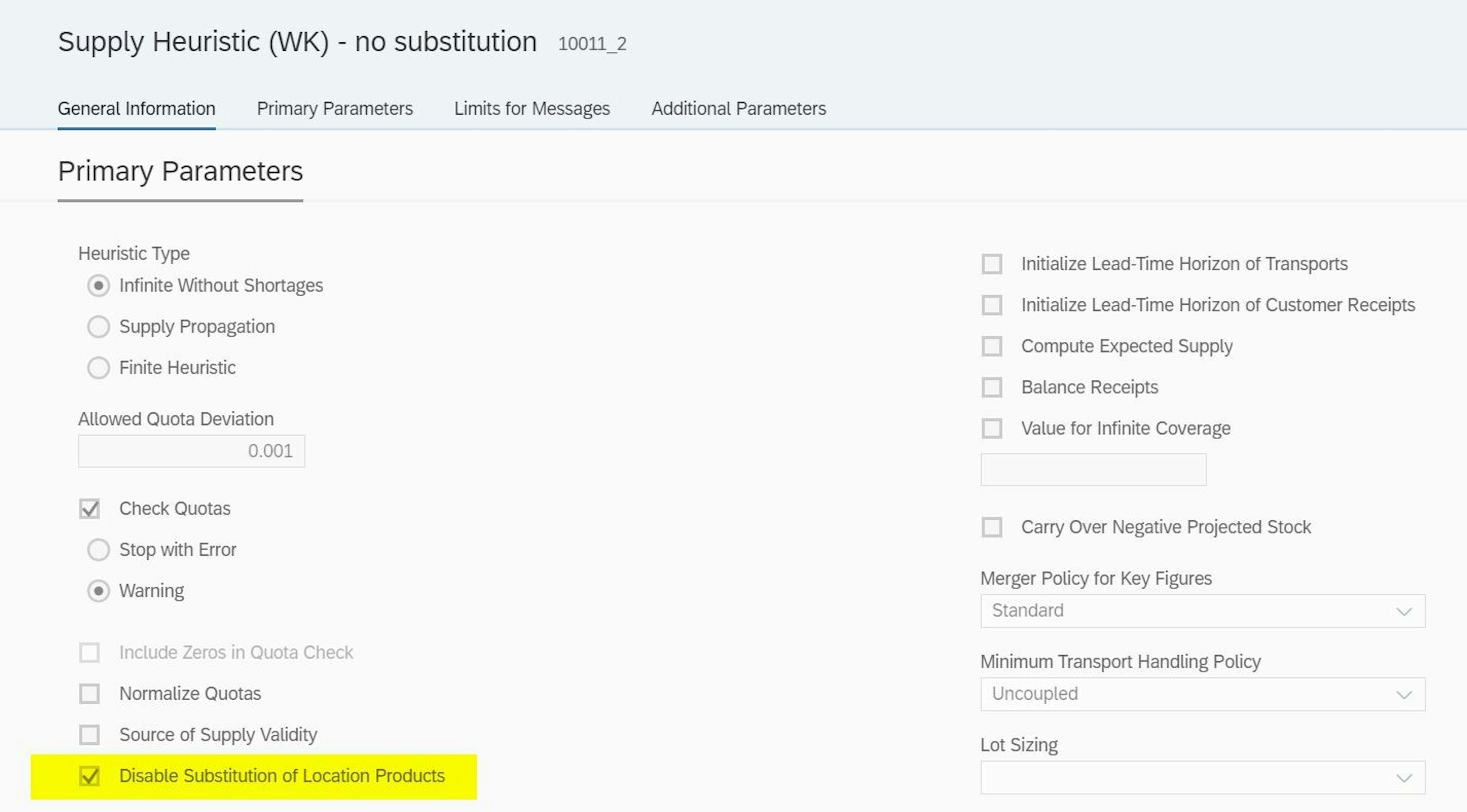
While the pre-2008 product substitution functionality is only available for products that are sold to market and can only be taken into account by the optimizer, the newest location product substitution is available with both the heuristic (infinite without shortages) and the optimizer. And while the optimizer can support more scenarios than the heuristic, you also need to define more parameters to make it work correctly – substitution and inventory holding cost rates need to be appropriately set up. In addition, the S&OP operators will consider this new functionality by default. So, if you do not wish to use it, you need to disable it in your S&OP operator profile.
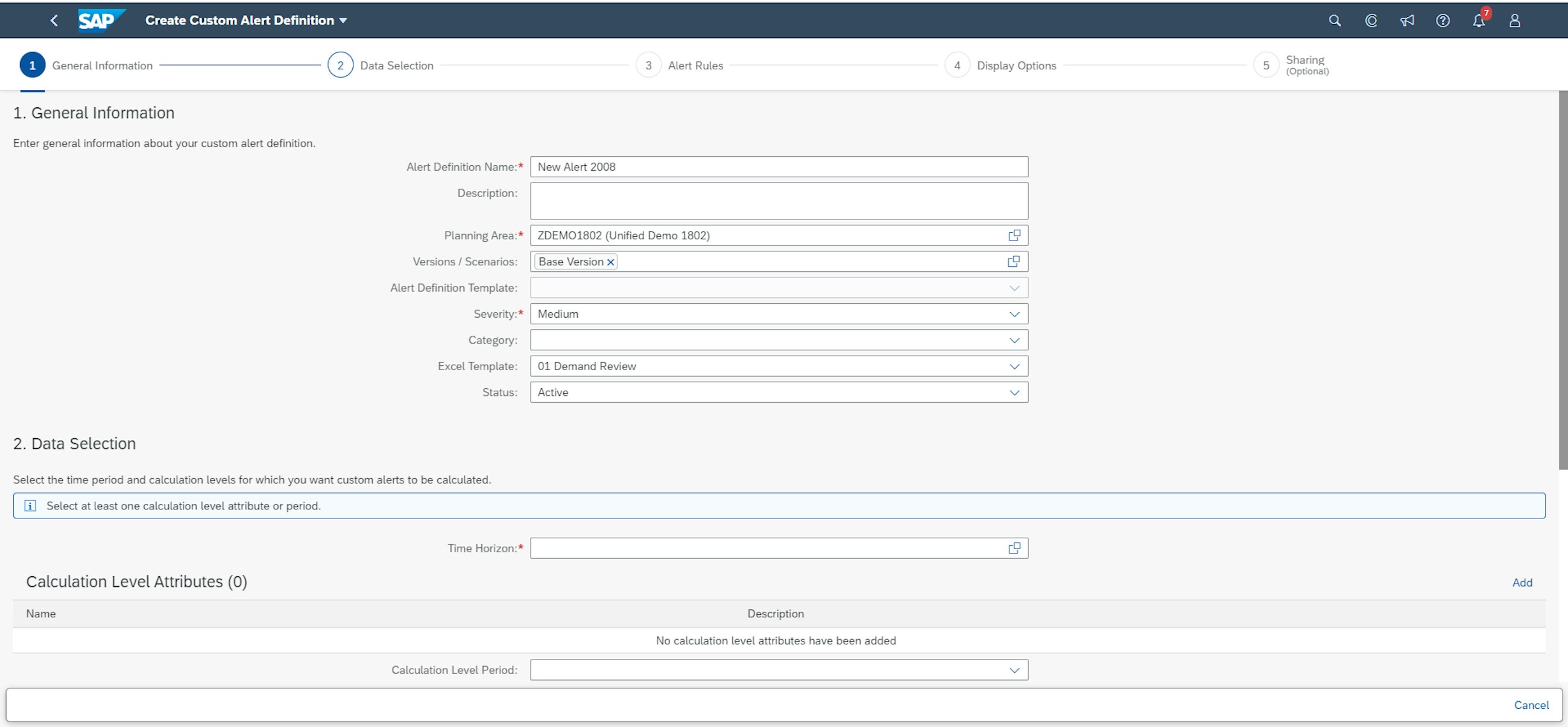
With the 2008 release, there is an upgrade to the “define and subscribe” to custom alerts app. The enhancements include a new design of the app but also enhancements that make it possible for you to create new types of alerts. The alerts enable you to identify critical issues in your supply chain and to take appropriate actions to solve them.
You can define one or more rules to your alerts in the alert definition, or you can define an alert definition template, where the static rules will be automatically filled out for you. The alert definition templates are created in the application job template app.
The rules you define compare a key figure to an absolute threshold value, or you can compare two key figure values by using the percentage value, e.g. if you want to review your forecast versus sales orders or deliveries. In addition to this, the new upgrade enables you to compare key figure values with an offset in the past or future from the selected time horizons. One last feature added to the upgrade is that you can now transport the alert definitions and alert overviews in the transport model entities application.
Be aware that the old application is marked as deprecated and will be deleted during the 2011 release.